Numerical Differentiation


Numerical differentiation is the process of finding the numerical value of a derivative of a given function at a given point. In general, numerical differentiation is more difficult than numerical integration. This is because while numerical integration requires only good continuity properties of the function being integrated, numerical differentiation requires more complicated properties such as Lipschitz classes. Numerical differentiation is implemented as ND[f, x, x0, Scale -> scale] in the Mathematica package NumericalCalculus` .

There are many applications where derivatives need to be computed numerically. The simplest approach simply uses the definition of the derivative





for some small numerical value of h<1

link of numerical methods (books)

http://books.google.com.co/books?id=armfeHpJIwAC&printsec=frontcover&dq=numerical+methods&source=gbs_similarbooks_s&cad=1#v=onepag

http://books.google.com.co/books?id=y77n2ySMJHUC&printsec=frontcover&dq=numerical+methods&source=gbs_similarbooks_s&cad=1#v=onepage&q&f=false

http://books.google.com.co/books?id=czHV-1bEFl0C&printsec=frontcover&dq=numerical+methods&source=gbs_similarbooks_s&cad=1#v=onepage&q=numerical%20methods&f=false

TAKING CARE OF OUR PLANET

CALCULATION OF ROOTS OF EQUATIONS
METHOD OF BISECTION

It is the oldest and most basic method of finding the roots of an equation. Is directly based on the theorem of Bolzano explained above. Involves taking an interval [x0, x1] such that f (x0) f (x1) <0,> Maxit), in which case you need to print an error message indicating that the method does not converge.

Two operations represented in the diagram in figure (3) require additional explanation:

The midpoint of the interval is calculated as in the workplace. It thus follows an overall strategy to make numerical calculations indicating that it is better to calculate a term adding a small amount of correction to a previously obtained approximation. For example, in a computer of limited accuracy, there are values x0 and x1 for which xm is calculated by leaving the interval [x0, x1].
The convergence () is calculated using the expression. Thus, the term represents the number of significant figures with which we obtain the result.

METHOD OF SUCCESSIVE APPROXIMATIONS


Given the equation f (x) = 0, the method of successive approximations replaced by an equivalent equation, x = g (x), defined in the form g (x) = f (x) + x. To find the solution, we start with an initial value x0 and compute a new approach x1 = g (x0). We replace the new value obtained and repeat the process. This leads to a succession of values, if it converges, will limit the solution of the problem.



















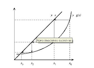
Figure (4) shows the geometric interpretation of the method. We start from an initial point x0 and compute y = g (x0). The intersection of this solution with the line y = x will give a new value x1 closer to the final solution.

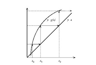
However, the method can easily diverge. It is easy to verify that the method can only converge if the derivative g '(x) is smaller in absolute value than unity (the slope of the line defined by y = x). An example of this case is shown in Figure (5). This condition, which a priori can be considered a severe restriction of the method, can be ignored easily. It is sufficient to choose the function g (x) as follows:


so that taking a proper value, we can always make g (x) satisfies the condition of the derivative.

















NEWTON METHOD


This method is part of an initial approximation x0 and obtains a better approximation, x1, given by the formula:
(29)


The above expression can be derived from a Taylor series expansion. Indeed, let r be a zero of f and an approximation ar x such that r = x + h. If f''exists and is continuous, by Taylor's theorem we have:


0 = f (r) = f (x + h) = f (x) + hf '(x) + O (h2) (30)


where h = r-x. If x is near ar (hes ie small), it is reasonable to ignore the term O (h2):


0 = f (x) + hf '(x) (31)


so we get the following expression for h:

(32)


From equation (32) and taking into account that r = x + h is easy to derive the equation.
















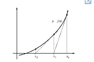
Newton's method has a simple geometric interpretation, as can be seen from the analysis of the figure (6). In fact, Newton's method is a linearization of the function, ie f is replaced by a line that contains the point (x0, f (x0)) and whose slope coincides with the derivative of the function at the point , f '(x0). The new approach to the root, x1, is obtained from the intercept of the linear function with the X-axis of ordinates.




Let's see how we can obtain equation (29) from what is said in the previous paragraph. The equation of the line through the point (x0, f (x0)) and slope f '(x0) is:


and - f (x0) = f '(x0) (x-x0) (33)


where, with y = 0 and solving for x we obtain the Newton-Raphson equation (29).









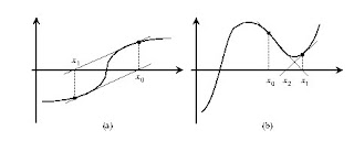
Newton's method is very fast and efficient since the convergence is quadratic (the number of significant digits doubles at each iteration). However, the convergence depends heavily on the form that function in the vicinity of the iteration. are two situations in which this method is not able to achieve convergence or converge to a point that is not a zero of the equation.




SECANT METHOD

The main disadvantage of Newton's method is that it requires knowing the value of the first derivative of the function at the point. However, the functional form of f (x) sometimes hampers the calculation of the derivative. In these cases it is more useful to use the secant method.
The secant method from two points (and not just one as the Newton method) and estimates the tangent (ie, the slope of the line) by an approach according to the expression:

(34)




Substituting this in equation (29) of Newton's method, we obtain the expression of the secant method gives us the next iteration point:

















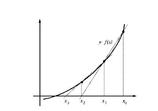
In the next iteration, we use the points x1 and x2para estimate a new point closer to the root of Eq (35). In figure (8) this method is represented geometrically.

In general, the secant method has the same advantages and limitations of the Newton-Raphson method described above.


METHOD OF FALSE POSITION



The method of false position is intended to combine the security of the bisection method with the speed of the secant method. This method, as with the bisection method stems from two points surrounding the root f (x) = 0, ie, two points x0 and x1tales that f (x0) f (x1) <0. The following approach, x2, is calculated as the X axis intersection with the line joining two points (using equation (35) of the secant method). The allocation of the new search interval is as in the bisection method: between the two intervals, [x0, x2] and [x2, x1], take that which satisfies f (x) f (x2) <0. Figure (9) is represented geometrically this method.















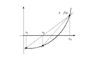
The choice guided the range represents an advantage over the secant method as it inhibits the possibility of a divergence of method. On the other hand and regarding the bisection method, greatly improves the choice of the interval (and not merely from the interval by half).










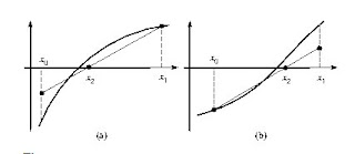
However, the method of false position has a very slow convergence towards the solution. Indeed, after starting the iterative process, one end of the interval tends to change (see Figure (9)). To circumvent this problem, we proposed a modification of the method, called Hamming method. Under this method, the approximation to a root is from the determination of the X axis intersection with the line joining the points (x0, f (x0) / 2) and (x1, f (x1)) if the function is convex in the interval or from the line joining the points (x0, f (x0)) and (x1, f (x1) / 2) if the function is concave in the interval. Figure (10) is plotted the Hamming method.




As mentioned, the Hamming method required to determine the concavity or convexity of the function in the interval of iteration. A relatively simple method to determine the curvature of the function is to evaluate the function at the midpoint of the interval, f (xm) (where xm is calculated as the bisection method).

MODELING

MODELING

In applied science, a mathematical model is one of the types of scientific models, which employs some form of mathematical formulas to express relationships, substantive propositions of facts, variables, parameters, entities and relationships between variables and / or entities or transactions, to study behavior of complex systems are difficult to observe situations in reality.

The meaning of fundamental mathematical mathematical model, however, is different. Specifically in mathematics work with formal models. A formal model for some mathematical theory is a set on which they have defined a set of unary relations, binary and trinary, which satisfies the propositions derived from axioms of set theory. The branch of mathematics that is required to examine systematically the properties of the models is the theory of models.

The term is also used mathematical modeling in graphic design when it comes to models of objects in 2D or 3D.

SOMETHING ABOUT MODELING

A model is a smart way or to organize, understand or explain something that happens, or believe may happen in the world. These are the ways or adopt guidelines to relate to anything at all, and here we are also included.

Model
Modeling is the process of creating models or ways to do or understand something. Each person has their ways or patterns of doing things and understanding the world. In the area of behavior modeling is concerned with identifying, understanding and re-create specific behaviors with which specific outcomes or at least create approximations to them.

Refer to our model has to do with the way in which we do things to adapt to the environment, ourselves and others. Modeling is make or model ways to do what we do or need to do in our lives and the world. They are ways to organize and relate to the world, are ways of understanding life and interact with reality, or what we have reality, and that's precisely where it is really important to have an accurate model and accurate, to approach and connect with the world properly.

PLEASE NOTE


* Without accurate and precise models we can not enjoy a successful life.
* We relate to the world from our model.
* A precise and exact model of successful performances.
* A model idle uncertain and erroneous actions.
* A person's culture is the set of modes of action with which he lives.
* Each one has its own model of the world, and although it is different from other people, we share and interact with them.
* Shaping our models or modes of action, we can direct our actions and enjoy life more effective, efficient and elegant.
* The purpose of modeling the behavior is to create a practical map for their conduct, so that it can play and get what we want from it.
* Emotions run behavior.
* It is modeled from the subtle observation of the behavior that you take as a model, is analyzed without breaking the model creates a map or summary of it and finally play.
* All models are inaccurate and fail to fully describe the world.

We can model a conscious or unconscious. Although most models that we have established operate without realizing-O we have inherited from the same society in which we operate, "we can create or shape a consciousness with adequate preparation new ones that open us new possibilities. Also improve, reform, refine, refine, refine, innovate, correct ... the existing, which finally emerge other than those originating models.


WE HAVE OUR SKILLS TO CREATE NATURAL MODELS.

We have models to create models, these in turn can be molded and extended to create more accurate models and efficient. Extend these skills consciously gives us a wide range of possibilities and added control for our lives. A real possibility and will actually improve our performance. Hence the importance of modeling our way of modeling.


MODEL TO CHANGE. For vital that our model is sufficiently useful and accurate, we need to be constantly remodeling them. Do not practice any skills will be lost. This is why we have to maintain and improve our abilities to model, if we want to have a way that allows us to better adapt to this changing world and live a more prosperous and successful.



Each model has its limits and set limits. A model is OK assume or believe their limits. The danger arises when one believes the world is the model. A model can describe only a small fraction of what exists. Provide better tools and distinctions allows us to transgress the boundaries of inaccurate models, extend and create rich models, accurate and less restrictive.



SOCIETY FOR MOVING OR BASED ON THEIR EXISTING MODELS.
Very few people go to transgress boundaries, to see whether they are really true. It is much more common for individuals engaged in search for evidence that the existing limits are real issues to which one cheer. Also it is to accept the prevailing social and wait if possible, than the general changes when they are hits, we transform.


The prevailing models in a society are closely connected with the beliefs and values of individuals of that society. For example: In the Middle Ages was the model that the earth was flat. No one except a few are devoted to questioning what all accepted by conviction, since the model was reasonable and obvious. The reality, possible or impossible, was organized from that model and the limitations were demarcated by the information that created it. Obviously this model was restricted as restricted information that was formed. To name something, the model did not contemplate the possibility that the earth was spherical because they had no notion of the "law of gravity" or "the law of universal gravitation." With this lack of information organized the world of that time

* One limitation is the result of the information the states.
* From the ideas that create a limitation, it is impossible to dispel.


MODEL TALK IS TALK OF ITS LIMITS.
The boundaries of a model is established from certain information that organizes the model. If you change or extend the information, process or dissipate and thus limiting the model

APPROXIMATIONS
The numerical methods are useful alternative procedures to solve math problems for which complicates the use of traditional analytical methods and, occasionally, are the only possible solution.
These are techniques by which a mathematical model is solved using only arithmetic operations, ... tedious arithmetic.
They are systematic techniques whose results are approximations of the true value that assumes the variable of interest, the consistent repetition of the technique, which is called iteration, is what you closer and closer to the desired value.


NUMERICAL APPROXIMATION

Numerical approximation is defined as X * a figure that represents a number whose exact value is X. To the extent that the number X * is closer to the exact value X, is a better approximation of that number
Examples:
3.1416 is a numerical ,approximation of π
2.7183 is a numerical approximation of e,
1.4142 is a numerical approximation of √2
0.333333 is a numerical approximation of one third.


SIGNIFICANT FIGURES
The measurements are normally done through instruments, such as a speedometer to measure the speed of a car, or an odometer to measure the distance covered.
The number of significant figures is the number of digits t, which can be used with confidence to measure a variable, for example, three significant figures on the speedometer and 7 significant figures on the odometer.
The zeros are included in a number are not always significant figures, for example, the numbers 0.00001845, 0.001845, 184 500 1845 and apparently have four significant figures, but would have to know the context in which they are working on each case, to identify how many and zeros which should be considered as significant figures.
The management of significant figures can develop criteria to detect how accurate are the results obtained and assess levels of accuracy and precision with which they are expressed some numbers such as √2, e or π .
Alternatively the number of significant figures, n is the number of digits in the mantissa, which indicates the number of numbers to consider, after the decimal point. In manual operations, the number of digits in the mantissa is still relevant, although it has been gradually displaced by the number of significant figures, by design, manage calculators and computers.


ACCURACY AND PRECISION
Accuracy refers to the number of significant figures represents a quantity.
Accuracy refers to the approach of a number or measure the numerical value is supposed to represent.
 is an irrational number, consisting of anExample: infinite number of digits; 3.141592653589793 ... , which may be an approximation π as good of considered which is its exact value. In considering the following approaches : π
π = 3.15 is vague and inaccurate.
π= 3.14 is accurate but imprecise.
π = 3.151692 is precise but inaccurate.
π = 3.141593 is accurate and precise.
The numerical methods should provide sufficiently accurate and precise solutions. The error term is used to represent both the inaccuracy and to measure the uncertainty in the predictions.

CONVERGENCE AND STABILITY
Convergence is defined as a numerical method ensuring that, when making a "good number" of iterations, the approximations obtained eventually move closer and closer to the true value sought.
To the extent that a numerical method requires fewer iterations than the other, to approach the desired value, is said to have a faster convergence.
Stability means of a numerical method the level of assurance of convergence and numerical methods is that some do not always converge and, on the other hand, diverge, ie away from the more desired result.
To the extent that a numerical method, to a very wide range of possibilities of mathematical modeling, it is safer to converge than the other, is said to have greater stability.
It is common to find methods that converge quickly, but they are very unstable and, in contrast, very stable models, but slow convergence.

SELECTION OF ALTERNATIVES
The use of numerical methods in engineering is not trivial, because it requires choosing between:
Several alternative numerical methods for each type of problem
Several technological tools
There are different ways to approach problems from one person to another, depending on:
The level of participation in the mathematical modeling of the problem
Ingenuity and creativity to confront and resolve
The ability to choose, according to criteria and experience

NMfP[1]

Nemerical Methods Julian

NMfP[1]